Chapter 1. Introduction
Who will benefit from this book?
Students who will find this book useful are those who have not systematically learned statistics or machine learning, but have had some exposure to basic statistical knowledge such as normal distribution, hypothesis testing, and are interested in finding data scientist jobs in a variety of areas. And practitioners with or without formal training in data science-related disciplines, who use data science in interdisciplinary areas, will find this book a useful addition. For example, I know a friend who learned statistics in college, more or less as applied mathematics that less emphasized data, computation, and storytelling, had found a remarkable resemblance between many data science methods with some concepts that she learned 20 years ago. She said if she could have a book that helps connect all the dots, and go through the materials with an easy-to-follow programming tool, it would help her move to a new field of work, as she is a physicist who is now working on genetics data.
We feel the same way. We have been working with medical doctors to diagnose surgical site infections using mobile phone images, with healthcare professionals to use hospital data to optimize the care process, with biologists and epidemiologists to understand the natural history of diseases, and with manufacturing companies to build Internet-of-Things, among others. The challenge of interdisciplinary collaboration is to cross boundaries and build new platforms. To embark on this adventure, a flexible understanding of our methods is important, as well as the skill of storytelling.
To help readers develop these skills, the style of the book highlights a combination of two aspects: technical concreteness and holistic thinking2 The chapters are named using different qualities of holistic thinking in decision-makings, including “Abstraction,” “Recognition,” “Resonance,” “Learning,” “Diagnosis,” “Scalability,” “Pragmatism,” and “Synthesis.”. Holistic thinking is the foundation of how we formulate problems and why we could trust our formulations, knowing that our formulations inevitably are only a partial representation of a real-world problem. Holistic thinking is also the foundation of communication between team members of different backgrounds. With a diverse team, things that make sense intuitively are important to build team-wide trust in decision-making. And technical concreteness is the springboard for us to jump into a higher awareness and understanding of the problem to make holistic decisions.
To begin our journey, first, let’s look at the big picture, the data analytics pipeline.
Overview of a data analytics pipeline
A typical data analytics pipeline consists of several major pillars. In the example shown in Figure 2, it has four pillars: sensor and devices, data preprocessing and feature engineering, feature selection and dimension reduction, and modeling and data analysis. While this is not the only way to present the diverse data pipelines in the real world, these pipelines more or less resemble this architecture.
Figure 2: Overview of a data analytics pipeline
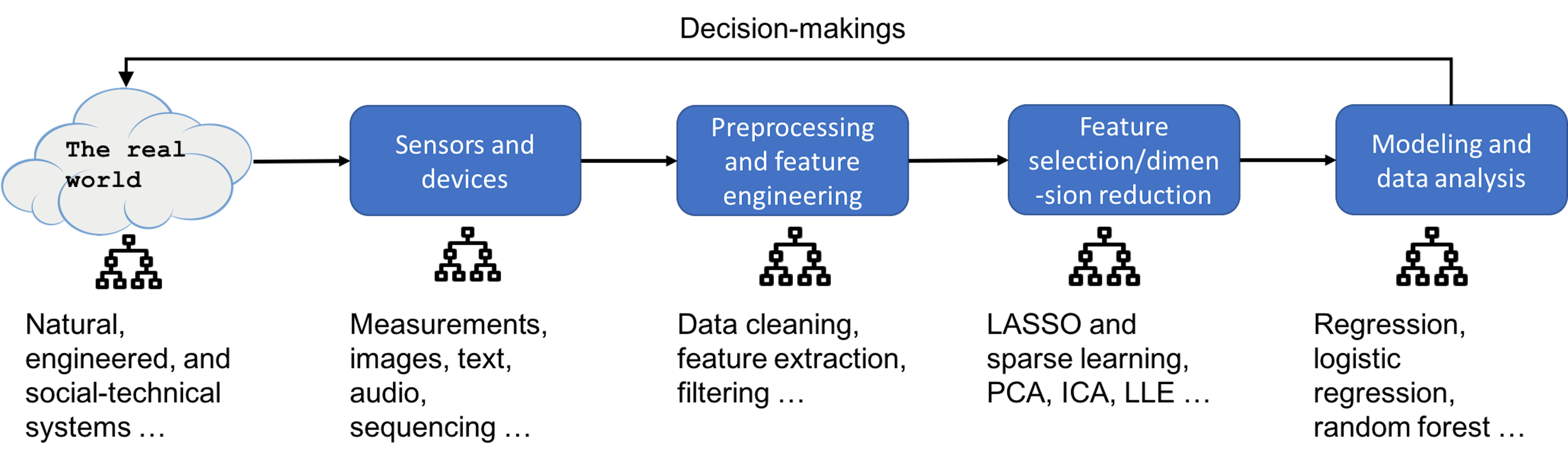
The pipeline starts with a real-world problem, for which we are not sure about the underlying system/mechanism, but we are able to characterize the system by defining some variables. Then, we could develop sensors and devices to acquire measurements of these variables3 These measurements, we call data, are objective evidences that we can use to explore the statistical principles or mechanistic laws regulating the system behaviors.. Before analyzing the data and building models, there is a step for data preprocessing and feature engineering. For example, some signals acquired by sensors are not interpretable or not easily compatible with human perceptions, such as the signal acquired by MRI scanning machines in the Fourier space. Data preprocessing also refers to removal of outliers or imputation of missing data, detection and removal of redundant features, to name a few. After data preprocessing, we may conduct feature selection and dimension reduction to distill or condense signals in the data and reduce noise. Finally, we conduct modeling and data analysis on the prepared dataset to gain knowledge and build models of the real-world system4 Prediction models are quite common, but other models for decision-makings, such as system modeling, monitoring, intervention, and control, can be built as well..
This book focuses on the last two pillars of this pipeline, the modeling, data analysis, feature selection, and dimension reduction methods. But it is helpful to keep in mind the big picture of a data analytics pipeline. Because in practice, it takes a whole pipeline to make things work.
Topics in a nutshell
Specific techniques that will be introduced in this book are shown below.
Data models (i.e., regression-based techniques)
Chapter 2: Linear regression, least squares estimation, hypothesis testing, R-squared, First Derivative Test, connection with experimental design, data-generating mechanism, history of adventures in understanding errors, exploratory data analysis (EDA)
Chapter 3: Logistic regression, generalized least squares estimation, iterative reweighted least squares (IRLS) algorithm, ranking (formulated as a regression problem)
Chapter 4: Bootstrap, data resampling, nonparametric hypothesis testing, nonparametric confidence interval estimation
Chapter 5: Overfitting and underfitting, limitation of R-squared, training dataset and testing dataset, random sampling, K-fold cross-validation, the confusion matrix, false positive and false negative, the Receiver Operating Characteristics (ROC) curve, the law of errors, how data scientists work with clients
Chapter 6: Residual analysis, normal Q-Q plot, Cook’s distance, leverage, multicollinearity, heterogeneity, clustering, Gaussian mixture model (GMM), the Expectation-Maximization (EM) algorithm, Jensen Inequality
Chapter 7: Support Vector Machine (SVM), generalize data versus memorize data, maximum margin, support vectors, model complexity and regularization, primal-dual formulation, quadratic programming, KKT condition, kernel trick, kernel machines, SVM as a neural network model
Chapter 8: LASSO, sparse learning, \(L_1\)-norm and \(L_2\)-norm regularization, Ridge regression, feature selection, shooting algorithm, Principal Component Analysis (PCA), eigenvalue decomposition, scree plot
Chapter 9: Kernel regression as generalization of linear regression model, local smoother regression model, k-nearest neighbor (KNN) regression model, conditional variance regression model, heteroscedasticity, weighted least squares estimation, model extension and stacking
Chapter 10: Deep learning, neural network, activation function, model primitives, convolution, max pooling, convolutional neural network (CNN)
Algorithmic models (i.e., tree-based techniques)
Chapter 2: Decision tree, entropy, information gain (IG), node splitting, pre- and post-pruning, empirical error, generalization error, pessimistic error by binomial approximation, greedy recursive splitting
Chapter 3: System monitoring reformulated as classification problem, real-time contrasts method (RTC), design of monitoring statistics, sliding window, anomaly detection, false alarm
Chapter 4: Random forest, Gini index, weak classifiers, the probabilistic mechanism about why random forests can create a strong classifier out of many weak classifiers, importance score, partial dependency plot
Chapter 5: Out-of-bag (OOB) error in random forest
Chapter 6: Residual analysis, clustering by random forests
Chapter 7: Ensemble learning, Adaboost, analysis of ensemble learning from statistical, computational, and representational perspectives
Chapter 10: Automations of pipelines, integration of tree models, feature selection, and regression models in
inTrees, random forest as a rule generator, rule extraction, pruning, selection, and summarization, confidence and support of rules, variable interactions, rule-based prediction
In this book, we will use lower case letters, e.g., \(x\), to represent scalars, bold face, lower case letters, e.g., \(\boldsymbol{x}\), to represent vectors, and bold face, upper case letters, e.g., \(\boldsymbol{X}\), to represent matrices.