Appendix: A Brief Review of Background Knowledge
Recall that in this book, we use lower case letters, e.g., \(x\), to represent scalars; bold face, lower case letters, e.g., \(\boldsymbol{x}\), to represent vectors; and bold face, upper case letters, e.g., \(\boldsymbol{X}\), to represent matrices.
The Normal Distribution
A distribution model characterizes the random behavior of a random variable. A random variable takes value from a predefined set, range, or a continuum, but not all values are taken with equal probabilities. How these probabilities are distributed is characterized by the distribution model. Before the computer age, for a distribution model to acquire a status of natural law it usually has an elegant geometric shape that comes with a delicate mathematical form, as many examples shown in Figure 5. As we have computers now doing a lot of computation, a distribution could be just an empirical histogram that has not yet found its explicit mathematical form. Whether or not this empirical form of distribution would repeat itself as a natural law remains to be seen. In practice, a competitive edge could be gained before you find scientific explanation, as long as it works.
In this book we will not have extensive coverage of distribution models. We will focus on normal distribution; but other than that, everything we learn about the normal distribution is also to help us extend beyond it and establish the concept of distribution as an abstract one.
A random variable \(x\) distributed as a normal distribution is denoted as
\[\begin{equation*} \small x \sim N\left(\mu, \sigma^{2}\right). \end{equation*}\]
The normal distribution has the mathematical form
\[\begin{equation*} \small N\left(\mu, \sigma^{2}\right) = \frac{1}{\sqrt{2\pi} \sigma}e^{-\frac{1}{2}(\frac{x - \mu}{\sigma})^2 }. \end{equation*}\]
If we multiply \(x\) with a constant \(a\), then
\[\begin{equation*} \small ax \sim N\left(a\mu, a^2\sigma^{2}\right). \tag{103} \end{equation*}\]
Extending the concept of distribution to \(p\)-dimensional space, we have the multivariate normal distribution (MVN) of vector \(\boldsymbol{x}\)
\[\begin{equation*} \small \boldsymbol{x} \sim MVN\left(\boldsymbol{\mu}, \boldsymbol{\Sigma}\right), \end{equation*}\]
where
\[\begin{equation*} \small \boldsymbol{\mu}=\left[ \begin{array}{c}{\mu_{1}} \\ {\mu_{2}} \\ {\vdots} \\ {\mu_{p}}\end{array}\right], \text { } \boldsymbol{\Sigma}=\left[ \begin{array}{cccc} {\sigma^2_{1}} & {\sigma_{12}} & {\cdots} & {\sigma_{1p}} \\ {\sigma_{21}} & {\sigma^2_{2}} & {\cdots} & {\sigma_{2p}} \\ {\vdots} & {\vdots} & {\vdots} & {\vdots} \\ {\sigma_{p1}} & {\sigma_{p2}} & {\cdots} & {\sigma^2_{p }}\end{array}\right], \end{equation*}\]
and
\[\begin{equation*} \small MVN\left(\boldsymbol{\mu}, \boldsymbol{\Sigma}\right) = \frac{1}{\sqrt{(2\pi)^p\det{\boldsymbol{\Sigma}}}}\exp\left({-\frac{1}{2}(\boldsymbol{x}-\boldsymbol{\mu})^T\boldsymbol{\Sigma}^{-1}}(\boldsymbol{x}-\boldsymbol{\mu})\right). \end{equation*}\]
To interpret the covariance matrix \(\boldsymbol{\Sigma}\), let’s look at an example where \(p=2\). Its covariance matrix is
\[\begin{equation*} \small \boldsymbol{\Sigma_1} = \left[ \begin{array}{cc} {\sigma^2_1} & {\sigma_{12}} \\ {\sigma_{21}} & {\sigma_2^2}\end{array}\right]. \end{equation*}\]
The element \(\sigma^2_1\) is the marginal variance of variable \(x_1\), \(\sigma^2_2\) is the marginal variance of variable \(x_2\), and \(\sigma_{12}\) that equals to \(\sigma_{21}\) is the covariance between \(x_1\) and \(x_2\).286 Covariance is closely related to the concept of correlation. For instance, denote the correlation between \(x_1\) and \(x_2\) as \(r\), which is defined as \(r = \frac{\sigma_{12}}{\sigma_1\sigma_2}\). It could be shown that \(r\) takes value from \(-1\) (i.e., perfect negative correlation) to \(1\) (i.e., perfect positive correlation). Note that this correlation concept is built on the normal distribution, and the correlation \(0\) doesn’t imply the two variables have no relationship in any possible form. Rather, it only implies that there is no linear relationship between the two.
Three examples of the covariance matrix are shown below
\[\begin{equation*} \small \boldsymbol{\Sigma_1} = \left[ \begin{array}{cc} {1} & {0} \\ {0} & {1}\end{array}\right], \text { } \boldsymbol{\Sigma_2} = \left[ \begin{array}{cc} {1} & {0.8} \\ {0.8} & {1}\end{array}\right], \text { } \boldsymbol{\Sigma_3} = \left[ \begin{array}{cc} {1} & {1} \\ {1} & {1}\end{array}\right]. \end{equation*}\]
The corresponding contour plots of the three bivariate normal distributions are shown in Figure 199.
If we add \(\boldsymbol{x}\) (i.e., \(\boldsymbol{x} \in R^{p \times 1}\)) with a constant vector \(\boldsymbol{a}\) (i.e., \(\boldsymbol{a} \in R^{p \times 1}\)), then
Figure 199: The contour plots of the three bivariate normal distributions

\[\begin{equation*} \small \boldsymbol{a + x} \sim MVN\left(\boldsymbol{a + \mu}, \boldsymbol{\Sigma}\right). \end{equation*}\]
If we multiply \(\boldsymbol{x}\) (i.e., \(\boldsymbol{x} \in R^{p \times 1}\)) with a constant \(\boldsymbol{a}\) (i.e., \(\boldsymbol{a} \in R^{p \times 1}\)), then
\[\begin{equation*} \small \boldsymbol{a^Tx} \sim MVN\left(\boldsymbol{a^T\mu}, \boldsymbol{a^T\Sigma a}\right). \end{equation*}\]
Matrix Operations
A matrix is a basic structure in data analytics that organizes data in a rectangular array, e.g., a matrix \(\boldsymbol{X} \in R^{p \times q}\) with \(p\) rows and \(q\) columns is
\[\begin{equation*} \small \boldsymbol{X}=\left[ \begin{array}{cccc} {x_{11}} & {x_{12}} & {\cdots} & {x_{1q}} \\ {x_{21}} & {x_{22}} & {\cdots} & {x_{2q}} \\ {\vdots} & {\vdots} & {\vdots} & {\vdots} \\ {x_{p1}} & {x_{p2}} & {\cdots} & {x_{pq}}\end{array}\right]. \end{equation*}\]
Matrix transposition. A matrix \(\boldsymbol{X} \in R^{p \times q}\) could be transposed into a matrix \(\boldsymbol{X}^T \in R^{q \times p}\), i.e.,
\[\begin{equation*} \small \boldsymbol{X}^T=\left[ \begin{array}{cccc} {x_{11}} & {x_{21}} & {\cdots} & {x_{q1}} \\ {x_{12}} & {x_{22}} & {\cdots} & {x_{q2}} \\ {\vdots} & {\vdots} & {\vdots} & {\vdots} \\ {x_{1p}} & {x_{2p}} & {\cdots} & {x_{qp}}\end{array}\right]. \end{equation*}\]
Matrix addition. Two matrices of the same dimensions could be added together entrywise, i.e., \(\boldsymbol{X} + \boldsymbol{Y}\) is defined as
\[\begin{equation*} \small \boldsymbol{X + Y}=\left[ \begin{array}{cccc} {x_{11}+y_{11}} & {x_{12}+y_{12}} & {\cdots} & {x_{1q}+y_{1q}} \\ {x_{21}+y_{21}} & {x_{22}+y_{22}} & {\cdots} & {x_{2q}+y_{2q}} \\ {\vdots} & {\vdots} & {\vdots} & {\vdots} \\ {x_{p1}+y_{p1}} & {x_{p2}+y_{p2}} & {\cdots} & {x_{pq}+y_{pq}}\end{array}\right]. \end{equation*}\]
Scalar multiplication: The product of a constant \(c\) and a matrix \(\boldsymbol{X} \in R^{p \times q}\) is computed by multiplying every entry of \(\boldsymbol{X} \in R^{p \times q}\) by \(c\), i.e.,
\[\begin{equation*} \small c\boldsymbol{X}=\left[ \begin{array}{cccc} {cx_{11}} & {cx_{12}} & {\cdots} & {cx_{1q}} \\ {cx_{21}} & {cx_{22}} & {\cdots} & {cx_{2q}} \\ {\vdots} & {\vdots} & {\vdots} & {\vdots} \\ {cx_{p1}} & {cx_{p2}} & {\cdots} & {cx_{pq}}\end{array}\right]. \end{equation*}\]
Matrix multiplication. Two matrices could be multiplied if the number of columns of the left matrix is the same as the number of rows of the right matrix, i.e., for \(\boldsymbol{X} \in R^{p \times q}\), it could be multiplied with any matrix that has \(q\) rows. Let’s say we have two matrices, \(\boldsymbol{X} \in R^{2 \times 3}\) and \(\boldsymbol{Y} \in R^{3 \times 2}\), the multiplication \(\boldsymbol{XY}\) is a matrix \(\in R^{2 \times 2}\), where
\[\begin{equation*} \small \boldsymbol{XY}=\left[ \begin{array}{cccc} {x_{11}y_{11}+ x_{12}y_{21}+ x_{13}y_{31}} & {x_{11}y_{12}+ x_{12}y_{22}+ x_{13}y_{32}} \\ {x_{21}y_{11}+ x_{22}y_{21}+ x_{23}y_{31}} & {x_{21}y_{12}+ x_{22}y_{22}+ x_{23}y_{32}}\end{array}\right]. \end{equation*}\]
Matrix derivative. Matrix derivative is a rich category that includes many situations. Readers may find a comprehensive coverage in a few books287 Harville, D.A., Matrix Algebra From a Statistician’s Perspective, Springer, 2000. or find a quick reference in online resources288 Petersen, K.B. and Pedersen, M.S., The Matrix Cookbook, online document (https://www.math.uwaterloo.ca/~hwolkowi/matrixcookbook.pdf).. Here, we mention a few examples that are related topics in this book.
Denote that \(y=f(\boldsymbol{X})\) is a scalar function of the matrix \(\boldsymbol{X} \in R^{p \times q}\). Then derivative of \(y\) with respect to the matrix \(\boldsymbol{X}\) is given by
\[\begin{equation*} \small \frac{\partial y }{\partial \boldsymbol{X}} = \left[ \begin{array}{cccc} \frac{\partial y }{\partial x_{11}} & \frac{\partial y }{\partial x_{12}} & {\cdots} & \frac{\partial y }{\partial x_{1q}} \\ \frac{\partial y }{\partial x_{21}} & \frac{\partial y }{\partial x_{22}} & {\cdots} & \frac{\partial y }{\partial x_{2q}} \\ {\vdots} & {\vdots} & {\vdots} & {\vdots} \\ \frac{\partial y }{\partial x_{p1}} & \frac{\partial y }{\partial x_{p2}} & {\cdots} & \frac{\partial y }{\partial x_{pq}}\end{array}\right]. \end{equation*}\]
Based on this definition, we can derive that
\[\begin{equation*} \small \frac{\partial \boldsymbol{a}^T\boldsymbol{x} }{\partial \boldsymbol{x}} = \boldsymbol{a}; \end{equation*}\]
\[\begin{equation*} \small \frac{\partial \boldsymbol{x}^T\boldsymbol{B}\boldsymbol{x} }{\partial \boldsymbol{x}} = (\boldsymbol{B} + \boldsymbol{B}^T)\boldsymbol{x}; \end{equation*}\]
\[\begin{equation*} \small \frac{\partial \boldsymbol{(x-a)}^T\boldsymbol{B}\boldsymbol{(x-a)} }{\partial \boldsymbol{x}} = 2\boldsymbol{B}\boldsymbol{(x-a)}; \end{equation*}\]
\[\begin{equation*} \small \frac{\partial \boldsymbol{(Ax+b)}^T\boldsymbol{W}\boldsymbol{(Cx+d)} }{\partial \boldsymbol{x}} = \boldsymbol{A}^T\boldsymbol{W}\boldsymbol{(Cx+d)} + \boldsymbol{C}^T\boldsymbol{W}\boldsymbol{(Ax+b)}. \end{equation*}\]
Matrix norm. The \(L_1\) norm of a vector \(\boldsymbol{x}\) is defined as
\[\begin{equation*} \small \lVert \boldsymbol{x} \rVert_1 = \sum_{i=1}^p \lvert x_i \rvert. \end{equation*}\]
The \(L_2\) norm of a vector \(\boldsymbol{x}\) is defined as
\[\begin{equation*} \small \lVert \boldsymbol{x} \rVert^2_2 = \sum_{i=1}^p x_i^2. \end{equation*}\]
Optimization
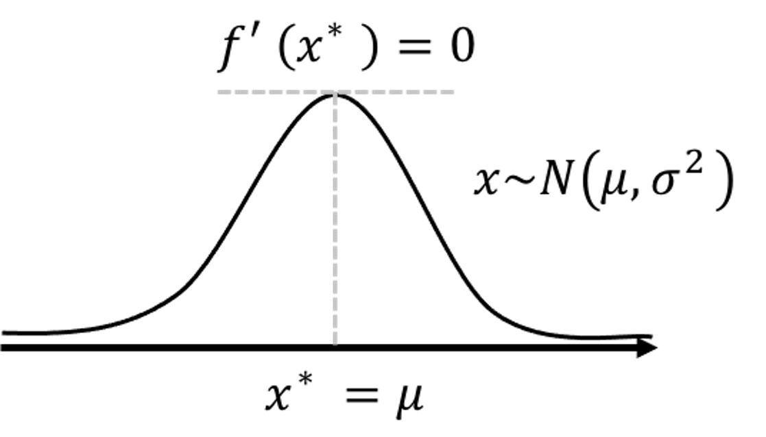 Figure 200: Illustration of the application of the First Derivative Test on the density function of a normal distribution to identify the location where the probability density is maximal.
The First Derivative Test, illustrated in Figure 10 in Chapter 2, is widely used in statistics and machine learning to find optimal solutions of a model formulation. Given a function \(f(x)\), the First Derivative Test finds the location \(x^*\) that leads to \(\frac{\partial f(x) }{\partial x} = 0\), i.e., denoted as \(f'(x^*)=0\). For instance, we can apply the First Derivative Test on the density function of a normal distribution to identify the location where the probability density is maximal289 That is, the mean \(\mu\).. An illustration of this application is shown in Figure 200.
The locations that are identified by the First Derivative Test may not be the global optimal points, as shown in Figure 21 in Chapter 2. On the other hand, it is relatively easy to use and is found to be quite effective in practice. Gradient-based optimization algorithms have been built on this concept to iteratively search for the locations where the first derivative could be set to zero. One such example is shown in Figure 31 in Chapter 3.